Pivot Table With Text in Values Area

Can you build a pivot table with text in the values area? Susan from Melbourne Florida has a text field and wants to see the before and after of that text.

Traditionally, you can not move a text field in to the values area of a pivot table.

However, if you use the Data Model, you can write a new calculated field in the DAX language that will show text as the result.

1. Make sure your data is Formatted as Table by choosing one cell in the data and pressing Ctrl + T. Make a note of the table name as shown on the Table Tools tab of the ribbon.
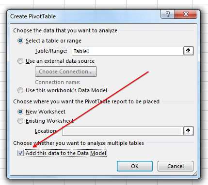
2. Insert, Pivot Table. Choose “Add This Data to the Data Model” while creating the pivot table.

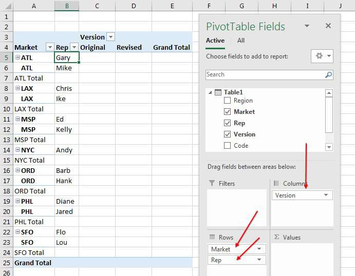
Drag fields to the Rows and Columns of the pivot table.

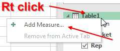
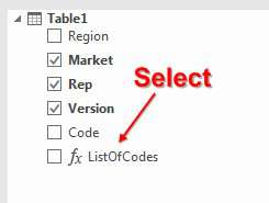
To add the text to the values area, you have to create a new special kind of calculated field called a Measure. Look at the top of the Pivot Table Fields list for the table name. Right-click the table name and choose Add Measure.

Note

If you do not have this option, then you did not choose Add This Data To The Data Model in step 2.

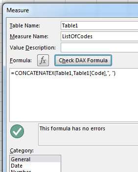
1. Type a field name of ListOfCodes
2. The formula is =CONCATENATEX(Table1,Table1[Code],", ")
3. Leave the format as General
4. Click Check DAX Formula to make sure there are no typos

Click OK. The new measure will appear in the field list.

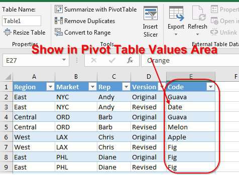
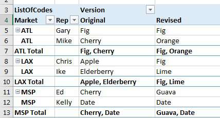
When you drag ListOfCodes to the Values area, you will see a list of codes for each cell in the values area.

Note

It is probably important to remove grand totals from this pivot table. Otherwise, the intersection of the Grand Total Row and Grand Total Column will list all of the codes in the table separated by columns. You can go to PivotTable Tools Design, Grand Totals, Off for Rows and Columns.

Amazingly, as you re-arrange the fields in Rows & Columns, the CONCATENATEX updates.

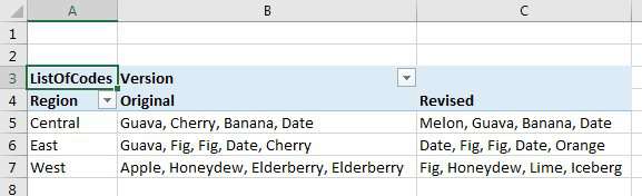
After using this method for a few weeks, I and others noticed that in some data sets, the concatenated values would contain duplicates, such as the Fig, Fig data shown in the East region above. Thanks to Rob Collie at PowerPivotPro.com, you can remove the duplicates by changing

=CONCATENATEX(Table1, Table1[Code], ”, “)

to

=CONCATENATEX(Values(Table1[Code]), Table1[Code], ", ")

The VALUES function returns a new table with the unique values found in a column.

Source : Pivot Table With Text in Values Area – Excel Tips – MrExcel Publishing

Burhan “OWL”

“The strongest among you is the one who controls his anger” – Muhammad SAW Hi, let me introduce myself. My name is Muhammad Burhanuddin Rabbani, but you can call me Burhan. I am a middle-aged man from Indonesia who is looking for a life partner. I have a Bachelor’s degree in Public Administration from Brawijaya University in Malang. However, my hobbies are more focused on photography and digital art, and I also dabble in web design and programming. Untuk gallery design bisa lihat di : https://www.burhan.web.id/artwork/ – – #burhan_owl #AvelineChrismonica

Burhan "OWL"

“The strongest among you is the one who controls his anger” – Muhammad SAW

Hi, let me introduce myself. My name is Muhammad Burhanuddin Rabbani, but you can call me Burhan. I am a middle-aged man from Indonesia who is looking for a life partner. I have a Bachelor’s degree in Public Administration from Brawijaya University in Malang. However, my hobbies are more focused on photography and digital art, and I also dabble in web design and programming.
Untuk gallery design bisa lihat di : https://www.burhan.web.id/artwork/
–
–
#burhan_owl #AvelineChrismonica

www.burhan.web.id